Step-by-step guide on Protein-Ligand MD simulation
Introduction
Importance of Protein ligand simulation
It helps to identify the potential drug candidates
It provides the detailed mechanism of how the drug binds to the target
They are faster and cheaper in comparison to experimental methods like X-ray and NMR
Prerequisites for Protein-ligand simulation
Docked Complex
Optimized protein without missing atoms or residues
Protein with proper charged residues
Optimized ligand molecule
Optimized protein and ligand is docked to find the optimal binding pose and binding affinity
The protein ligand complex with the favorable binding pose and binding energy is taken to simulation to study the time-dependent behavior of protein-ligand complex
Softwares required
Steps in protein-ligand simulation
Data Collection
Select the best protein-ligand complex after docking
Separate the protein ligand complex through the following commands
Select the best protein-ligand complex after docking
Separate the protein ligand complex through the following commands
| grep UNL 3HTB.pdb > jz4.pdb |
Here, UNL represents ligand molecule
jz4.pdb : ligand molecule
Additionally we need to remove the water molecules like below:
| grep -v HOH 3HTB.pdb > 3HTB_clean.pdb |
Removes any other atoms apart from the amino-acids. HOH represents the water molecule in this case
3HTB_clean.pdb : The docked protein alone
Protein topology creation
This step provides required information for the simulation software to calculate the forces and energies acting on each atom
| gmx pdb2gmx -f 3HTB_clean.pdb -o 3HTB_processed.gro -ignh |
Here, pdb2gmx : Converts input file from pdb format to gmx (gromacs format)
-f : input file name; o: output file name
-ignh: Ignores hydrogen atom in the protein and pdb2gmx adds hydrogen based on the field selected
This command will ask the user to select the forcefield as given below
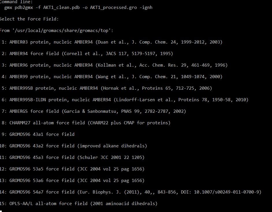
In this case, CHARMM27 is selected (option 8) . In all-atom force field, each atom including hydrogen is represented and parameter is assigned. In contrast united atom force field will combine the non-polar hydrogens with their parent atoms.
All atom force field will offer higher accuracy while studying molecular interactions like hydrogen bond, Van der waal and electrostatic interaction. It requires high computation power and time.
In next step, software will ask to select the water model
Water model is a mathematical representation of water molecules
It is essential for studying the protein folding and ligand binding
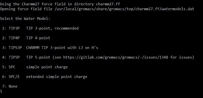
In this case,
TIP3P : Transferable Intermolecular Potential is selected
Water molecule is represented as three interaction sites
All the water models are rigid body water models where the bond angle and bond length remains unchanged during simulation
It is widely used in biomolecular simulations and is commonly used with AMBER, CHARMM and OPLS force field
TIP3P and SPC requires less computational power and is commonly used in protein-ligand simulations
Output files generated
Topology file (.top)
It contains topology of the system like atom types, charge, bond length between atoms, bond angle, dihedral angles of the atom
Gromacs file (.gro)
Gromacs compatible co-ordinate file contains the atomic co-ordinates of all protein residues and rebuilt hydrogen atoms based on the selected force field
Position restraint file (posre.itp)
It contains parameters to restrain the position of selected atoms during energy minimization
Next task.....
Ligand topology creation
Gromacs contain predefined forcefield parameters such as bond length, bond angle and torsion angle for standard amino acids, nucleotide sequences alone. Ligands with non-standard atoms requires alternate option for topology creation.
| ACPYPE : Amber-99SB-ILDN Swissparam : Charmm27 CGENFF : Charmm37 |
Obabel conversion
Before we begin to parameterize the ligand, we need to convert the ligand file from pdb to mol2 file, with adding H atoms through open-babel. This can be achieved through your below command:
| obabel jz4.pdb -O jz4.mol2 -h |
Then we need to fix the bonds through running the perl script, via below command:
| perl sort_mol2_bonds.pl jz4.mol2 jz4_fix.mol2 |
Now we need to upload this jz4_fix.mol2 file to Swiss param, which will generate the parameter files for ligand molecule, required for us to integrate with Gromacs to perform MD simulation.
- Simply upload our latest jz4_fix.mol2 file to Swiss Param website.
- Choose MMFF based approach.
- Press
Launch Parameterizeto submit to Swiss param. - Download the tar file, and you will find the jz4_fix.itp and jz4_fix.pdb files inside the directory.
- First, copy the
jz4_fix.pdbto the current working directory, where we run protein-ligand MD simulation. - Open this file jz4_fix.itp, and copy the contents of
[ atomtypes ]and[ pairtypes ]and paste it in a new file namedjz4.prmand save them. - Now again open the file jz4_fix.itp, except the content of
[ atomtypes ]and[ pairtypes ], copy everything and create a new file namedjz4.itp, and save it. - Now transfer these two files ->
jz4.prmandjz4.itpto current working directory where you run Protein-Ligand MD Simulation.
Now, open your topol.top file, and include the jz4.prm after the charmm27.ff/forcefield.itp file, as indicated below.
; Include forcefield parameters #include "charmm27.ff/forcefield.itp" ; Include ligand parameters #include "jz4.prm" [ moleculetype ] ; Name nrexcl Protein_chain_A 3 |
Similarly, include the jz4.itp file between the posre.itp and charmm27.ff/tip3p.itp file in your topol.top as indicated below:
One last thing, at the end of topol.top file, you will notice it contains information about the different molecules contained in the system. Since we are planning to incorporate ligand file into our system, we need to include it like below:
Complex building
Now, we need to generate Gromacs format for ligand from PDB we obtained from Swiss param results. This is exactly the same way as we did for protein at the first step. This can be achieved by simply running the below command.
| gmx editconf -f jz4_fix.pdb -o jz4.gro |
Now we need to merge the structure of both Protein and Ligand, to make them as single complex.
To achieve this, open the Protein file in gromacs format (i.e 3HTB_processed.gro). Copy all the contents of the file, and paste it in new file named complex.gro file.
Now, open the ligand file (i.e jz4.gro), you will see below content:
Glycine aRginine prOline Methionine Alanine Cystine Serine 22 1LIG C7 1 2.154 -2.723 -0.414 1LIG C8 2 2.203 -2.677 -0.537 1LIG C9 3 2.264 -2.552 -0.545 1LIG C10 4 2.275 -2.474 -0.430 1LIG C11 5 2.166 -2.645 -0.300 1LIG C12 6 2.227 -2.519 -0.306 1LIG C4 7 2.427 -2.410 -0.004 1LIG C13 8 2.253 -2.443 -0.179 1LIG C14 9 2.396 -2.472 -0.138 1LIG OAB 10 2.338 -2.351 -0.438 1LIG H 11 2.362 -2.451 0.073 1LIG H1 12 2.414 -2.301 -0.008 1LIG H2 13 2.531 -2.432 0.022 1LIG H3 14 2.108 -2.821 -0.408 1LIG H4 15 2.195 -2.739 -0.625 1LIG H5 16 2.304 -2.516 -0.639 1LIG H6 17 2.131 -2.683 -0.204 1LIG H7 18 2.183 -2.475 -0.101 1LIG H8 19 2.236 -2.336 -0.195 1LIG H9 20 2.412 -2.580 -0.133 1LIG H10 21 2.465 -2.432 -0.213 1LIG H11 22 2.337 -2.316 -0.348 0.00000 0.00000 0.00000 |
Copy the contents from 1LIG and paste everything except the last line - which indicates the size of the box.
So your final complex.gro file should look something like below:
| LYSOZYME 2614 1MET N 1 0.556 -1.596 -0.893 1MET H1 2 0.522 -1.511 -0.855 1MET H2 3 0.520 -1.608 -0.986 1MET H3 4 0.527 -1.673 -0.836 ...... ...... ...... ...... 163ASN C 2612 0.621 -0.740 -0.126 163ASN OT1 2613 0.624 -0.616 -0.140 163ASN OT2 2614 0.683 -0.703 -0.011 1LIG C7 1 2.154 -2.723 -0.414 1LIG C8 2 2.203 -2.677 -0.537 1LIG C9 3 2.264 -2.552 -0.545 1LIG C10 4 2.275 -2.474 -0.430 1LIG C11 5 2.166 -2.645 -0.300 1LIG C12 6 2.227 -2.519 -0.306 1LIG C4 7 2.427 -2.410 -0.004 1LIG C13 8 2.253 -2.443 -0.179 1LIG C14 9 2.396 -2.472 -0.138 1LIG OAB 10 2.338 -2.351 -0.438 1LIG H 11 2.362 -2.451 0.073 1LIG H1 12 2.414 -2.301 -0.008 1LIG H2 13 2.531 -2.432 0.022 1LIG H3 14 2.108 -2.821 -0.408 1LIG H4 15 2.195 -2.739 -0.625 1LIG H5 16 2.304 -2.516 -0.639 1LIG H6 17 2.131 -2.683 -0.204 1LIG H7 18 2.183 -2.475 -0.101 1LIG H8 19 2.236 -2.336 -0.195 1LIG H9 20 2.412 -2.580 -0.133 1LIG H10 21 2.465 -2.432 -0.213 1LIG H11 22 2.337 -2.316 -0.348 5.99500 5.19182 9.66100 0.00000 0.00000 -2.99750 0.00000 0.00000 0.00000 |
One last thing before we move further. We need to update the total number of atoms present in complex.gro file through updating at the top after protein, which currently contains 2614, it should be added with 22 atoms of ligand to finally obtain 2636:
| LYSOZYME 2636 1MET N 1 0.556 -1.596 -0.893 1MET H1 2 0.522 -1.511 -0.855 1MET H2 3 0.520 -1.608 -0.986 ..... ..... ..... 1LIG H9 20 2.412 -2.580 -0.133 1LIG H10 21 2.465 -2.432 -0.213 1LIG H11 22 2.337 -2.316 -0.348 5.99500 5.19182 9.66100 0.00000 0.00000 -2.99750 0.00000 0.00000 0.00000 |
Now we are done with all the process related to creating the complex.gro file. Hope you all succeed in creating it too!
Box creation and Solvent addition
Now, Create the solavtion box for the protein-ligand complex
| gmx editconf -f complex.gro -o newbox.gro -c -d 1.0 -bt cubic |
editconf : Used while editing the co-ordinate file
f: Input ; o: Output file name
c: Centres protein in box; -d 1.0 : Places 0.1 nm away from the edges of the protein to box.
bt : Box type : Cubic. Other options like dodecahedron or triclinic can also be explored.
The complx_box.gro can be visualized in visualization software like pymol to visualize the box
| gmx solvate -cp newbox.gro -cs spc216.gro -p topol.top -o solv.gro |
cp: Configuration of protein in complex_box.gro
cs: Solvent configuration
Output file solv.gro will now contain the solvent molecules and can be visualized.
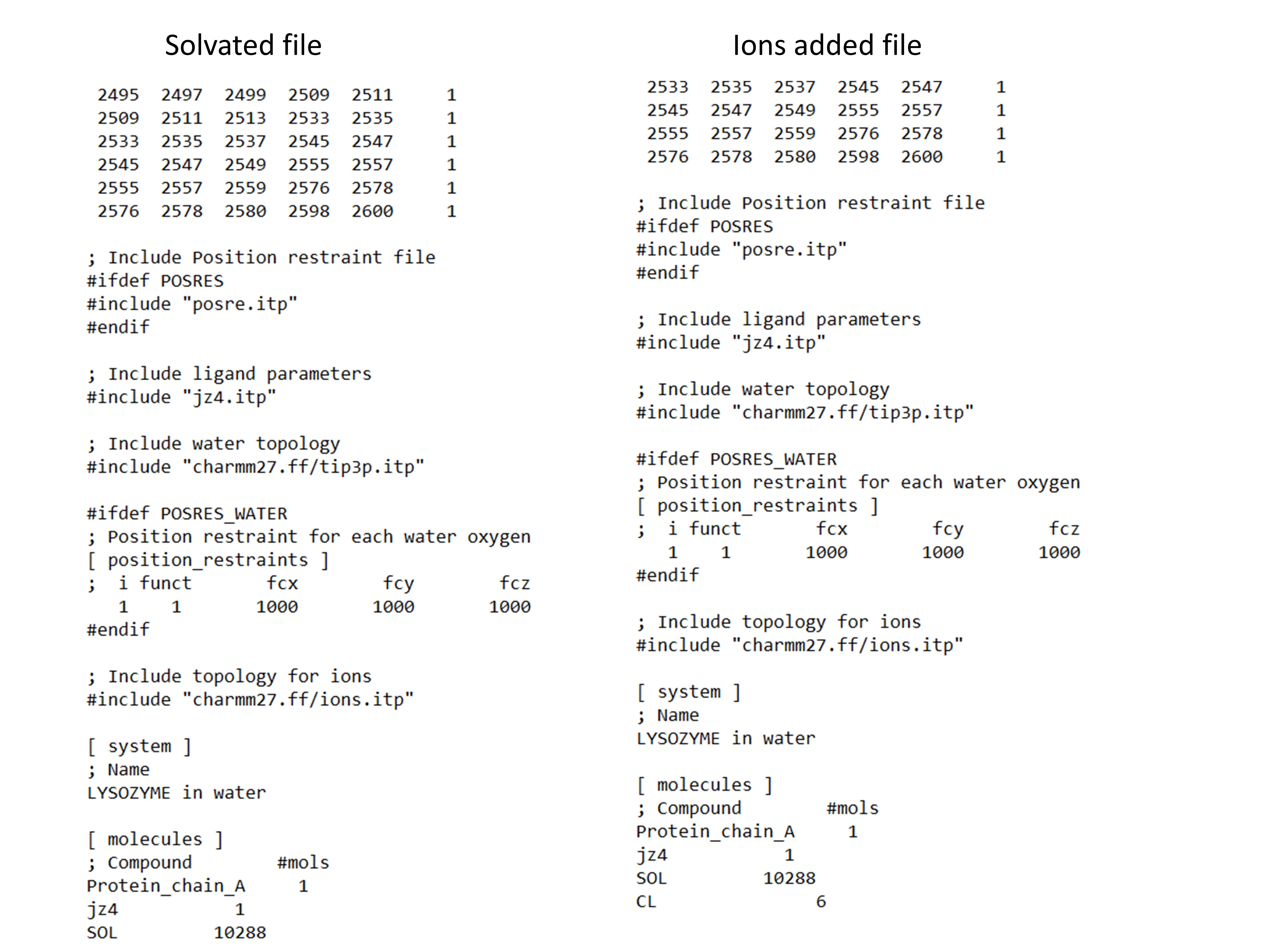
The topol.top file also automatically added with the information about solvent molecules as given in the image at the end
Adding Ions
Ions are added to the system. Ions.mdp is obtained here
| gmx grompp -f ions.mdp -c solv.gro -p topol.top -o ions.tpr |
grompp: Process the co-ordinate files and topol.top to generate atomic level input (ions.tpr) in order to add ions
| gmx genion -s ions.tpr -o solv_ions.gro -p topol.top -pname NA -nname CL -neutral |
Explanation for above command is:
genion : tool process topol.top by removing water and adding ions
ions.tpr is generated from the previous step
pname : name of positive ion
nname: name of negative ion
The net charge of the protein is neutralized and specific ion concentration can also be added on the basis of study
The above command will prompts for what molecule to be replaced with ions, select SOL by typing the appropriate number in the prompt.
Energy Minimization
To perform energy minimization, you need to have em.mdp file downloaded from the official gromacs tutorial.
Now run the below two commands:
gmx grompp -f em.mdp -c solv_ions.gro -p topol.top -o em.tpr gmx mdrun -v -deffnm em |
You will see energy minimization taking place with Gromacs.
NVT Equilibration
Restraining the ligand
gmx make_ndx -f jz4.gro -o index_jz4.ndx
| gmx genrestr -f jz4.gro -n index_jz4.ndx -o posre_jz4.itp -fc 1000 1000 1000 |
It will prompt you for selection, choose the newly created index group - System_&_!H* - mostly it will be numbered at 3.
Now we need to include this posre_jz4.itp file in our topol.top file, closely after we have added jz4.itp as below:
; Ligand position restraints #ifdef POSRES #include "posre_jz4.itp" #endif ; Include ligand parameters #include "jz4.itp" ; Ligand position restraints #ifdef POSRES #include "posre_jz4.itp" #endif ; Include water topology #include "charmm27.ff/tip3p.itp" |
So, we added posre_jz4.itp file to be included in topol.top file as indicated above, between the ligand parameters and water topology file.
Now run the below command, it will prompt for selection like:
| gmx make_ndx -f em.gro -o index.ndx ... 0 System : 47615 atoms 1 Protein : 2614 atoms 2 Protein-H : 1301 atoms 3 C-alpha : 163 atoms 4 Backbone : 489 atoms 5 MainChain : 651 atoms 6 MainChain+Cb : 803 atoms 7 MainChain+H : 813 atoms 8 SideChain : 1801 atoms 9 SideChain-H : 650 atoms 10 Prot-Masses : 2614 atoms 11 non-Protein : 45001 atoms 12 Other : 22 atoms 13 LIG : 22 atoms 14 CL : 6 atoms 15 Water : 44973 atoms 16 SOL : 44973 atoms 17 non-Water : 2642 atoms 18 Ion : 6 atoms 19 Water_and_ions : 44979 atoms nr : group '!': not 'name' nr name 'splitch' nr Enter: list groups 'a': atom '&': and 'del' nr 'splitres' nr 'l': list residues 't': atom type '|': or 'keep' nr 'splitat' nr 'h': help 'r': residue 'res' nr 'chain' char "name": group 'case': case sensitive 'q': save and quit 'ri': residue index |
When it prompts for selection like above, choose
> 1 | 13 > q
Now, download the nvt.mdp file from official gromacs. Before you can directly use this for your work, you need to update the tc-grps in your mdp file like tc-grps = Protein_LIG Water_and_ions to achieve our desired "Protein Non-Protein" effect.
This above change has to be performed in all the three mdp files, nvt.mdp, npt.mdp and md.mdp.
| gmx grompp -f nvt.mdp -c em.gro -r em.gro -p topol.top -n index.ndx -o nvt.tpr gmx mdrun -deffnm nvt -v |
NPT Equilibration
From now on, running NPT equilibration is quite simple and straight forward.
You just download the npt.mdp file from official gromacs website, and modified the tc-grps as above, and execute the two below commands one-by-one.
From now on, running NPT equilibration is quite simple and straight forward.
You just download the npt.mdp file from official gromacs website, and modified the tc-grps as above, and execute the two below commands one-by-one.
gmx grompp -f npt.mdp -c nvt.gro -t nvt.cpt -r nvt.gro -p topol.top -n index.ndx -o npt.tpr gmx mdrun -deffnm npt |
MD Simulation
gmx grompp -f md.mdp -c npt.gro -t npt.cpt -p topol.top -n index.ndx -o md_0_10.tpr gmx mdrun -deffnm md_0_10 -v |
Post-trajectory Analysis
It centers the molecule of interest in the simulation box
Fix broken molecules that may have been split across the box edges due to periodic boundary conditions (PBC).
"PBC artifacts, such as molecules appearing broken or jumping across box boundaries, are corrected.
| gmx trjconv -s md_0_10.tpr -f md_0_10.xtc -o md_0_10_center.xtc -center -pbc mol -ur compact |
Select Protein, press enter
Select System, press enter
MD-Analysis
Protein - RMSD
RMSD is a measure used to quantify the difference between two structures, typically in molecular dynamics (MD) simulations, to assess how much a structure deviates from a reference structure over time (initial structure).
Evaluates the overall stability of the systems
Provides insight into the stability of the protein backbone and how it is affected by ligand binding
A low RMSD indicates that the protein structure is stable and remains close to its native conformation during the simulation
Focusing on the backbone reduces noise caused by flexible side chains, providing a clearer picture of the protein’s overall structural dynamics
Root Mean Square Deviation
| gmx rms -s md_0_10.tpr -f md_0_10_center.xtc -n index.ndx -o protein_rmsd.xvg -tu ns |
Select Backbone
again
Select Backbone
protein_rmsd.xvg is generated and is visualized using Xmgrace in linux and Qtgrace in Windows
Protein_RMSF
Root Mean Square Fluctuation
- The RMSF values provide insight into the flexibility of each residue in the protein over the course of the simulation. Typically, loop regions in proteins tend to exhibit higher fluctuations due to their dynamic nature, whereas regions involved in secondary structures, such as α-helices and β-sheets, show lower fluctuations, indicating structural stability
| gmx rmsf -s md_0_10.tpr -f md_0_10_center.xtc -o protein_rmsf.xvg -res |
Select C-alpha and press enter
.xvg is generated
Radius of gyration
Rg measures the distribution of the atoms in the protein relative to its center of mass over time. A lower and stable Rg indicates that the protein maintains a compact and stable structure during the simulation, while significant fluctuations or a higher Rg value suggest the protein might be unfolding or becoming less compact
| gmx gyrate -s md_0_10.tpr -f md_0_10_center.xtc -o gyrate.xvg |
Select Protein and press enter
Hydrogen bond
| gmx hbond -s md_0_10.tpr -f md_0_10_center.xtc -n index.ndx -num hbond.xvg -tu ns |
Select Protein and press enter
Select LIG and press enter
hbond.xvg is created for further analysis
Protein-ligand simulations are powerful tools in drug discovery, providing insights into binding interactions, stability, and dynamics at the molecular level. By leveraging these simulations, researchers can predict binding affinities, optimize lead compounds, and accelerate the development of novel therapeutics. As computational methods continue to advance, protein-ligand simulations will play an increasingly vital role in modern drug design, bridging the gap between in silico predictions and experimental validation.
Every interaction begins with a bond — in science, as in life.